sleephealth <- read.csv("C:/Users/Jaxso/Downloads/Sleep_health_and_lifestyle_dataset.csv")DANL Project
Data-Driven Mastery: Unlocking Business Potential
1 Introduction
The following dataframe was used for this project 😴
2 Data
The data.frame sleephealth contains a subset of the fuel economy data that the EPA makes available on https://kaggle.com/. It comprises 400 rows and 13 columns, covering a wide range of variables related to sleep and daily habits. It includes variables such as gender, age, occupation, sleep duration, quality of sleep, physical activity level, stress levels, BMI category, blood pressure, heart rate, daily steps, and the presence or absence of sleep disorders. 🛏️
2.1 Summary Statistics
mpg <- ggplot2::mpgskim(sleephealth) %>%
select(-n_missing)| Name | sleephealth |
| Number of rows | 374 |
| Number of columns | 13 |
| _______________________ | |
| Column type frequency: | |
| character | 5 |
| numeric | 8 |
| ________________________ | |
| Group variables | None |
Variable type: character
| skim_variable | complete_rate | min | max | empty | n_unique | whitespace |
|---|---|---|---|---|---|---|
| Gender | 1 | 4 | 6 | 0 | 2 | 0 |
| Occupation | 1 | 5 | 20 | 0 | 11 | 0 |
| BMI.Category | 1 | 5 | 13 | 0 | 4 | 0 |
| Blood.Pressure | 1 | 6 | 6 | 0 | 25 | 0 |
| Sleep.Disorder | 1 | 4 | 11 | 0 | 3 | 0 |
Variable type: numeric
| skim_variable | complete_rate | mean | sd | p0 | p25 | p50 | p75 | p100 | hist |
|---|---|---|---|---|---|---|---|---|---|
| Person.ID | 1 | 187.50 | 108.11 | 1.0 | 94.25 | 187.5 | 280.75 | 374.0 | ▇▇▇▇▇ |
| Age | 1 | 42.18 | 8.67 | 27.0 | 35.25 | 43.0 | 50.00 | 59.0 | ▆▆▇▃▅ |
| Sleep.Duration | 1 | 7.13 | 0.80 | 5.8 | 6.40 | 7.2 | 7.80 | 8.5 | ▇▆▇▇▆ |
| Quality.of.Sleep | 1 | 7.31 | 1.20 | 4.0 | 6.00 | 7.0 | 8.00 | 9.0 | ▁▇▆▇▅ |
| Physical.Activity.Level | 1 | 59.17 | 20.83 | 30.0 | 45.00 | 60.0 | 75.00 | 90.0 | ▇▇▇▇▇ |
| Stress.Level | 1 | 5.39 | 1.77 | 3.0 | 4.00 | 5.0 | 7.00 | 8.0 | ▇▃▂▃▃ |
| Heart.Rate | 1 | 70.17 | 4.14 | 65.0 | 68.00 | 70.0 | 72.00 | 86.0 | ▇▇▂▁▁ |
| Daily.Steps | 1 | 6816.84 | 1617.92 | 3000.0 | 5600.00 | 7000.0 | 8000.00 | 10000.0 | ▁▅▇▆▂ |
2.2 Sleep Duration by Ocupation
The following boxplot shows how the mean sleep duration (Sleep.Duration) varies by occupation (Occupation) 😴 🛏️ .
mean_sleep_job <- sleephealth %>%
  group_by(Occupation) %>%
  summarize(
    n = n(),
    sleep_mean = mean(Sleep.Duration, na.rm = TRUE)
  ) %>%
  arrange(desc(n))
mean_sleep_job
# A tibble: 11 × 3
Occupation n sleep_mean
<chr> <int> <dbl>
1 Nurse 73 7.06
2 Doctor 71 6.97
3 Engineer 63 7.99
4 Lawyer 47 7.41
5 Teacher 40 6.69
6 Accountant 37 7.11
7 Salesperson 32 6.40
8 Scientist 4 6
9 Software Engineer 4 6.75
10 Sales Representative 2 5.9
11 Manager 1 6.9 ggplot( data = mean_sleep_job, mapping = aes(x = Occupation, y = sleep_mean)) +
geom_bar(stat = "identity") +
theme(axis.text.x = element_text(
angle = -45,
hjust = 0,
vjust = 1
))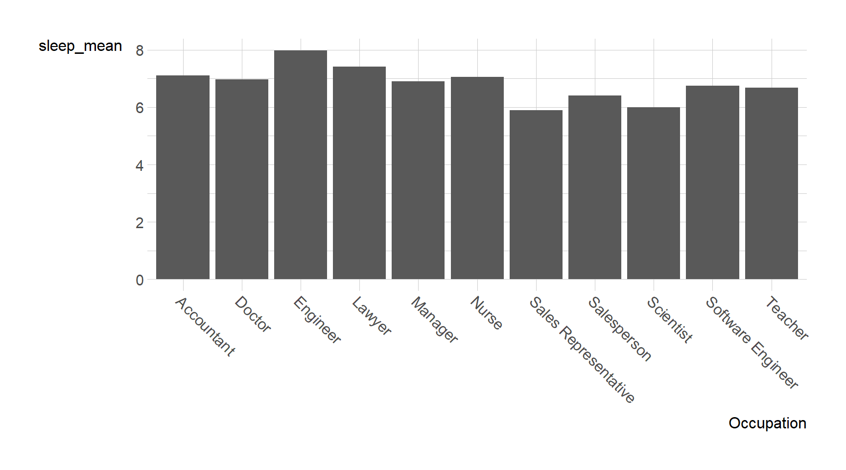
The bar graph represents the mean sleep duration amongst all the presented occupations in the ‘sleephealth’ dataset. After putting the data into a ggplot figure, it was found that engineer’s, on average, have the highest mean sleep duration at about 8 hours per night, and sales representative’s had the lowest mean sleep duration at just under 6 hours a night.
2.3 Effect of Physical Activity and Sleep Duration on Stress
This ggplot shows the effect of someone’s sleep duration (‘Sleep.Duration’) and level of physical activity (‘Physical.Activity.Level’) on their stress levels (‘Stress.Level’) 😠 😄 .
ggplot(sleephealth, aes(x = Sleep.Duration, y = Physical.Activity.Level, color = Stress.Level)) +
  geom_point() +
  labs(title = "Effect of Physical Activity and Sleep Duration on Stress",
       x = "Sleep Duration",
       y = "Physical Activity Level",
       color = "Stress Level") +
  theme(plot.title = element_text(size = 10))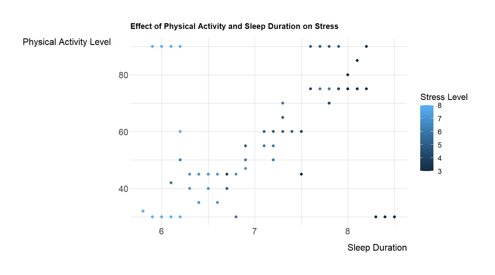
The above scatter plot visualizes the relationship between sleep duration and physical activity level in the ‘sleephealth’ dataset, with stress levels represented by color. Some interesting findings that were found was that a higher sleep duration and level of physical activity resulted in lower overall stress levels, while higher stress levels were a result of the inverse.
2.4 Sleep Duration and Quality of Sleep Among Varying Sleep Disorders
This ggplot shows the effect of different sleep disorders (‘Sleep.Disorder’) on the subjects’ quality of sleep (‘Quality.of.Sleep’) and overall sleep duration (‘Sleep.Duration’).
ggplot(sleephealth, aes(x = Sleep.Duration, y = Quality.of.Sleep, color = Quality.of.Sleep)) +
  geom_point() +
  facet_wrap(~ Sleep.Disorder) +
  labs(title = "Scatter Plot of Sleep Duration vs Quality of Sleep",
       x = "Sleep Duration",
       y = "Quality of Sleep",
       color = "Quality of Sleep") +
  scale_color_gradient(low = "blue", high = "red") +
  theme(plot.title = element_text(size = 12))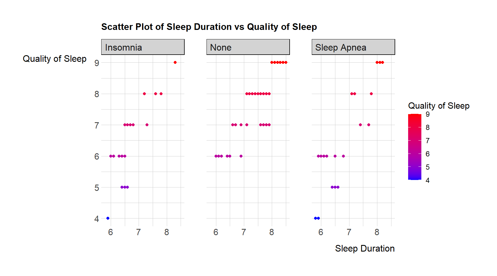
The scatterplots shown above outlines the ‘Quality.of.Sleep’ and “Sleep.Duration’ by varying ‘Sleep.Disorder’s shown within the ’sleephealth’ dataset. After compliling the ggplot, it was intersting to find that the three scatterplots showed a similar pattern amongst their data points, and that people with no sleep disorder didnt have a quality of sleep below ~6, even if they slept for the minimum number of hours.
2.5 Effect of Age and Occupation on BMI
The following ggplot represents how BMI (‘BMI.Category’) is different depending on each job (‘Occupation’) and varying ages (‘Age’).
ggplot(sleephealth, aes(x = BMI.Category, y = Age, fill = Occupation)) +
  geom_tile(color = "white") +
  scale_fill_brewer(palette = "Set2") +
  labs(title = "Heatmap of BMI Category by Age and Occupation",
       x = "BMI Category",
       y = "Age",
       fill = "Occupation") +
  theme_minimal() +
  theme(axis.text.x = element_text(angle = 45, hjust = 1))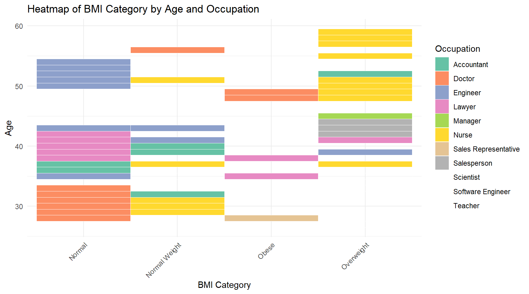
The heatmap shown above represents two variables, ‘Occupation’ and ‘Age’, and their effect on ‘BMI.Category’ within the ‘sleephealth’ data frame. Some interesting things to note from the plot is that, most engineers of all ages were within a normal weight range, and that all the salespersons that were subjected to the data are between the ages of 40-45 years old and also overweight.